Groundtruth data for Computer Vision with Blender

In the video below you can see the sequence of a car driving in a city scene and braking. The layers I rendered out for groundtruth data are the rendered image with the boundingbox of the car (top left), the emission layer ( shows the brakelights when they start to emit light, top right ), the optical flow (lower left), and the depth of each pixel in the world scene ( lower right).

Setting up groundtruth rendering for depth, saving and reading it again

After you have composed your scene, switch to the Cycles rendering engine, and enable the render-passes in the properties-view (under render-layers) you plan on saving as ground-truth information. In this case, I selected the Z-layer, which represents the depth of the scene:

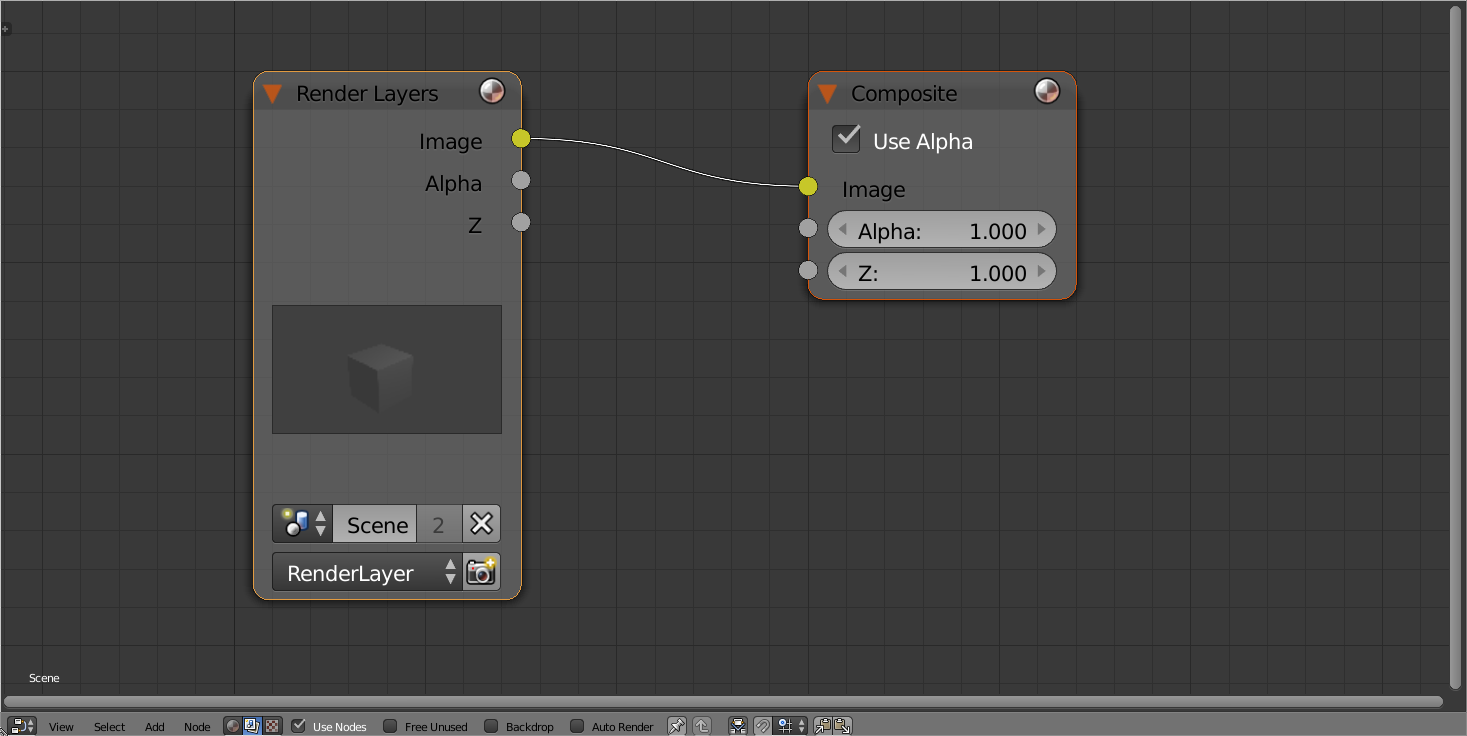
Now open the Node-editor-view, display the Compositing-Nodetree and put a checkmark at „Use Nodes“, it should look like this:

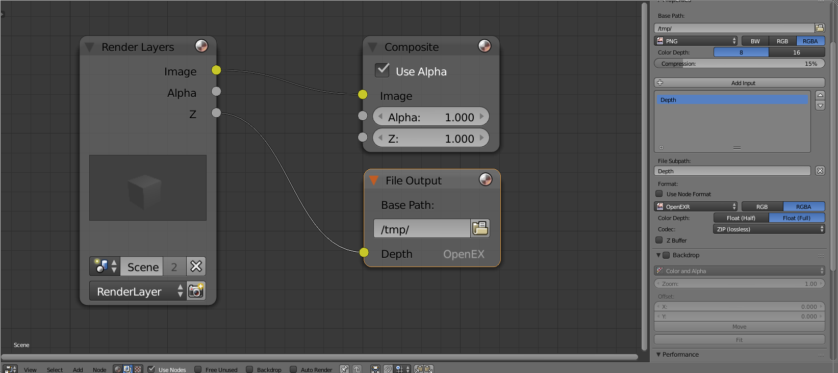
Hit „T“, and in the „output“-tab, select „File Output“. Connect it to the Z-output of the render-layers-node. Hit „N“ while the File-Output-node is selected, enter an appropriate File-subpath as name for the data (I chose „Depth“ here), and depending on your usecase, change the output format. As I am expecting float-values that are not constrained to 0-255, I will save the data in the OpenEXR-format:

After rendering ([F12]), we have a file called /tmp/Depth0001.exr. It can be read and displayed using python:

#!/usr/bin/python                                                                                                             

'''
author: Tobias Weis
'''

import OpenEXR
import Imath
import array
import numpy as np
import csv
import time
import datetime
import h5py
import matplotlib.pyplot as plt

def exr2numpy(exr, maxvalue=1.,normalize=True):
    """ converts 1-channel exr-data to 2D numpy arrays """                                                                    
    file = OpenEXR.InputFile(exr)

    # Compute the size
    dw = file.header()['dataWindow']
    sz = (dw.max.x - dw.min.x + 1, dw.max.y - dw.min.y + 1)

    # Read the three color channels as 32-bit floats
    FLOAT = Imath.PixelType(Imath.PixelType.FLOAT)
    (R) = [array.array('f', file.channel(Chan, FLOAT)).tolist() for Chan in ("R") ]

    # create numpy 2D-array
    img = np.zeros((sz[1],sz[0],3), np.float64)

    # normalize
    data = np.array(R)
    data[data > maxvalue] = maxvalue

    if normalize:
        data /= np.max(data)

    img = np.array(data).reshape(img.shape[0],-1)

    return img

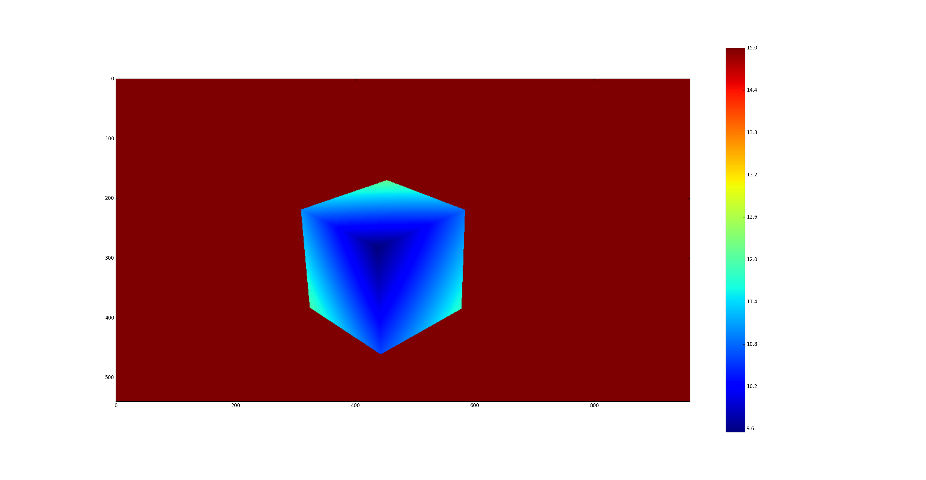
depth_data = exr2numpy("Depth0001.exr", maxvalue=15, normalize=False)

fig = plt.figure()
plt.imshow(depth_data)
plt.colorbar()
plt.show()

The output of this script on the default-scene looks like this:

Setting up groundtruth rendering for optical flow (speed vector), saving and reading it again

Create a scene with an object and a camera in it, then set keyframes for the camera (right-click on the location-values and select „Insert keyframe“). In the example below, I moved the camera 2m in its forward-direction over three frames. As you can see, the render-layer „Vector“ is enabled and like in the example above, I connected it to a File Output node and saved it in OpenEXR format.

If you now set your End-Frame (bottom panel), you can hit animate, and cycles will happily render the images and vector-maps to /tmp/. The following code-snippet will calculate any interesting informations about the optical flow for you.

Important information: The flow-values are saved in the R/G-channel of the output-image, where the R-channel contains the movement of each pixel in x-direction, the G-channel the y-direction. The offsets are encoded from the current to the previous frame, so the flow-information from the very first frame will not yield usable values. Also, in blender the y-axis points upwards. (The B/A-channels contain the offsets from the next to the current frame).

import array
import OpenEXR
import Imath
import numpy as np
import cv2

def exr2flow(exr, w,h):
  file = OpenEXR.InputFile(exr)

  # Compute the size
  dw = file.header()['dataWindow']
  sz = (dw.max.x - dw.min.x + 1, dw.max.y - dw.min.y + 1)

  FLOAT = Imath.PixelType(Imath.PixelType.FLOAT)
  (R,G,B) = [array.array('f', file.channel(Chan, FLOAT)).tolist() for Chan in ("R", "G", "B") ]

  img = np.zeros((h,w,3), np.float64)
  img[:,:,0] = np.array(R).reshape(img.shape[0],-1)
  img[:,:,1] = -np.array(G).reshape(img.shape[0],-1)

  hsv = np.zeros((h,w,3), np.uint8)
  hsv[...,1] = 255

  mag, ang = cv2.cartToPolar(img[...,0], img[...,1])
  hsv[...,0] = ang*180/np.pi/2
  hsv[...,2] = cv2.normalize(mag,None,0,255,cv2.NORM_MINMAX)
  bgr = cv2.cvtColor(hsv,cv2.COLOR_HSV2BGR)

  return img, bgr, mag,ang

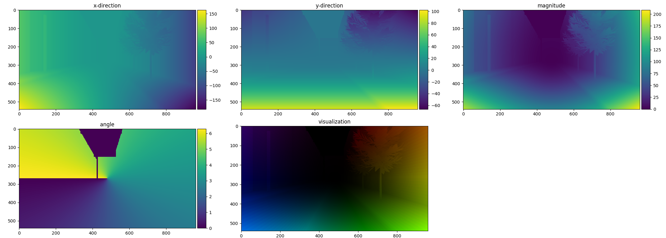
We can now use (and plot these informations), img contains the x/y-offsets in pixels, and by using opencvs cartToPolar-function we can calculate magnitude (absolute offset) and according angles for each pixels.
Finally, we can convert everything to a nice-looking color-image by first using the HSV (hue, saturation, value) colorspace, setting the hue to the angle, saturation to full, and the value to the magnitude:

Further layers to generate groundtruth data

Besides depth information, we can also generate groundtruth data for other modalities:

• Object/Material index: Can be used to generate pixel-accurate annotations of objects for semantic segmentation tasks, or simply computing bounding boxes for IOU measures
• Normal: Can be used to generate pixel-accurate groundtruth data of surface normals
• Vector: Will show up as „Speed“ in the node editor, contains information for optical flow between two frames in a sequence
• Emit: Pixel-accurate information of emssion-properties.